Data Analysis Software Details
The Data Analysis software tool enables you to Display, Analyze, Discriminate and Report one or multiple gravity calculations from the raw drop tower drop data.
The “Data Analysis” window has 3 main user interface regions. These regions can be quickly accessed with the buttons below.
The Upper Left Region is where the data is selected.
The Lower Left Region contains all the data analysis and reporting push buttons.
The Graphing Region is to the right of both these regions. This region contains a tabbed display of 10 different plots that correspond to a specific data analysis step.
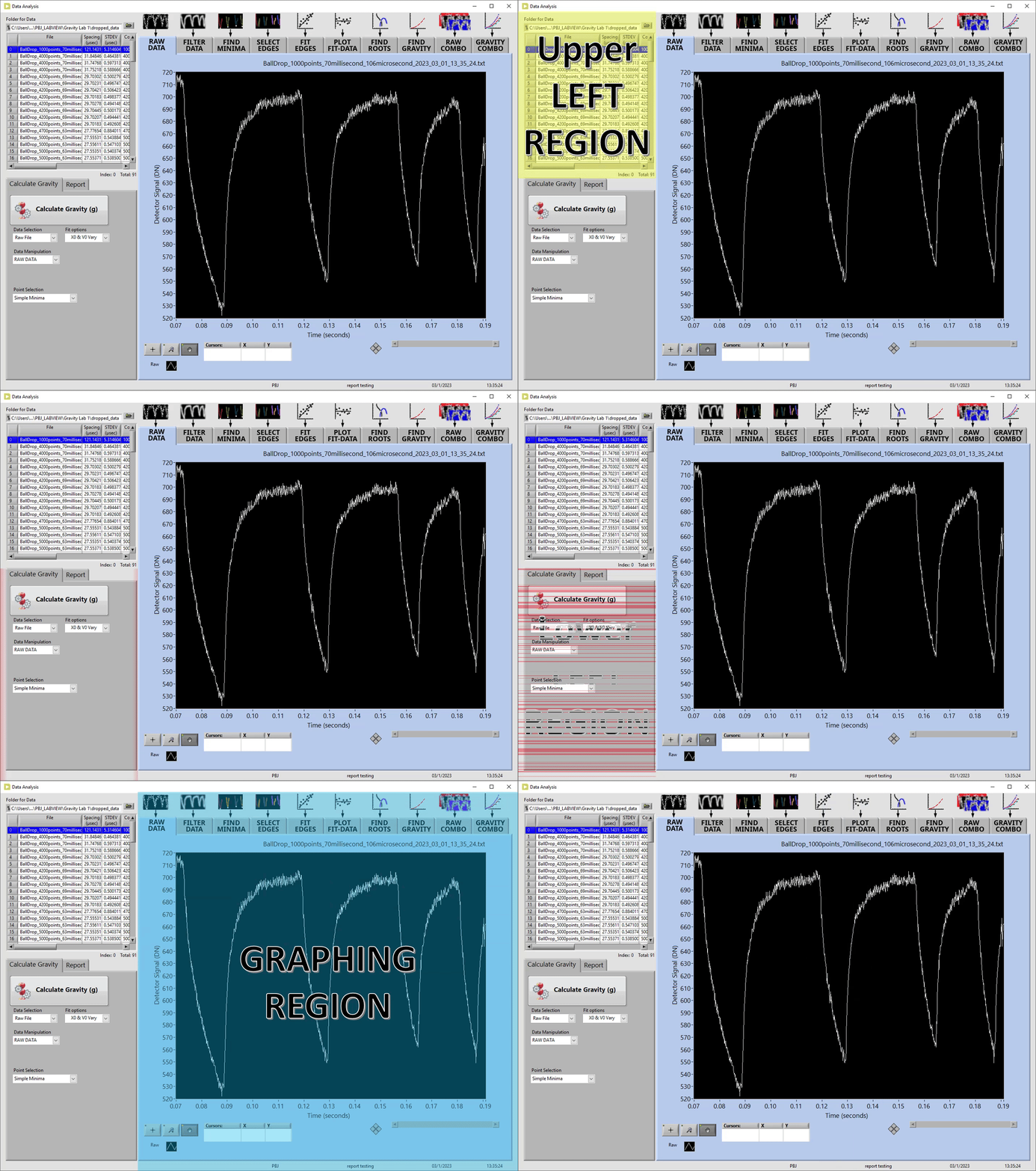
Upper Left Region
The upper left region consists of two controls. The folder selection control and a multi-column list-box control.
When this software tool is opened, the folder control will point to the default data drop folder location, and the multi-column list-box will display the contents of this folder.
The two following selections will detail these controls, and their right click options.
The “Folder for Data” control is operated by pushing the folder button on its right.
When this is done, a “Select Folder” window will appear allowing you to navigate to a folder of your choosing.
When you push the “Select Folder” button in this window, all the files in the displayed folder with a *.txt extension will be displayed int the multi-column list-box below this control.
All files with a *.txt extension are assumed to contain raw drop data. Therefore, all other files types are ignored.
If the folder contains non *.txt files a popup window of a flashing cloud will appear that displays the number of files being ignored.
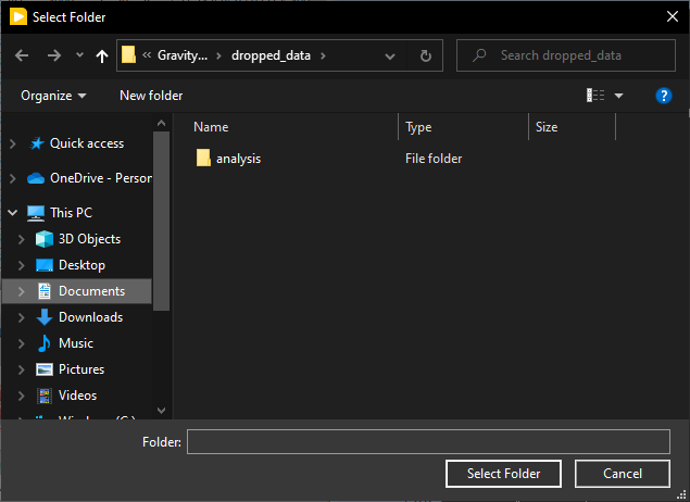
It is important to note that this LabView “Select Folder” window can be confusing, because it does not display any files only folders. Therefore when looking for a folder with specific files in it you may think they are missing, because this looks like a normal file browsing window. I did not chose this functionality, but I believe this is to prevent file selection when you are only supposed to select a folder.

You can right click on this folder control to get two useful options. The “explore folder” option opens the folder with the windows file explorer. This is useful if you want to see what is in the folder without effecting the multi-column list-box. The “reload folder” options is a quick way to re-read the current folder to the multi-column list-box without having to open the “Select Folder” window.
The multi-column list-box is a feature rich control in this data analysis window with two main purposes. The first purpose of this control is to quickly review the data in a given folder. The second purpose is to organize the data that you want to analyze.
At the start of the Data Analysis software, the multi-column list-box is activated and the currently highlighted row is plotted in the RAW DATA tab. When the multi-column list-box is activated, the Up and Down arrows can be used to quickly change the row selected thereby changing the current file that is plotted in the RAW DATA tab. You can also use your mouse to select a specific row.
The multi-column list-box will loose focus/activation when you click somewhere else in the “Data Analysis” window. To re-activate the multi-column list-box, you can click on it with your mouse our use the Page Down button as a shortcut.
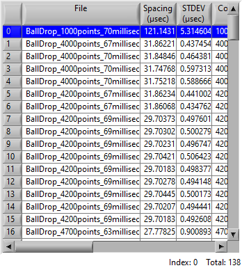
There are a total of 6 columns in the multi-column list-box that give the user additional information about each drop file. The contents of each column are detailed in the table below where columns 2 through 5 all require a properly named header for the drop file.
| Column # | Column Content |
|---|---|
| 1 | Data file names |
| 2 | Point to point spacing in microseconds (µs). |
| 3 | Variation of the point to point spacing measured as the Standard Deviation (STDEV) in microseconds (µsec) |
| 4 | Total number of data points. |
| 5 | Delay in milliseconds(ms) before the first data point is collected when the ball is dropped. |
| 6 | Folder path for current data file |
The multi-column list-box aids in organization through the use of the delete button and right-click options.
The delete button will remove the highlighted file from this list, but not the actual file in the folder.
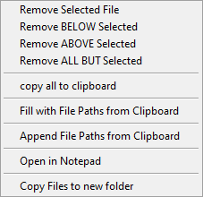
Right clicking on the multi-column list box control gives you 9 additional options. With these options, you are able to remove files in this list, add files to this list, copy this list, view a specific file in notepad, and copy all the files in this control to another folder.
The table below details what you can achieve with each option.
| Right-Click Option | Explanation |
|---|---|
| Remove Selected File | Remove the highlighted file from the multi-column list-box |
| Remove BELOW Selected | Remove every file below the highlighted file from the multi-column list-box |
| Remove ABOVE Selected | Remove every file above the highlighted file from the multi-column list-box |
| Remove ALL BUT Selected | Remove every file but the highlighted file from the multi-column list-box |
| copy all to clipboard | Copy the contents of the multi-column list-box to the clipboard in a tab delimited format |
| Fill with File Paths from Clipboard | The multi-column list-box is filled with the clipboard. The clipboard must contain the full path to a *.txt file separated by an end of line delimiter. |
| Append File Paths from Clipboard | The multi-column list-box is appended with the clipboard. The clipboard must contain the full path to a *.txt file separated by an end of line delimiter. |
| Open in Notepad | The currently highlighted file is opened in notepad.exe |
| Copy Files to new folder | All the file in the multi-column list-box are copied to a folder of your choosing. |
If any of the file paths do not exist, or do not have a *.txt extension, a popup window of a flashing cloud will appear that displays the number of files being ignored, how many are missing the *.txt extension and how many do not exist.
Lower Left Region
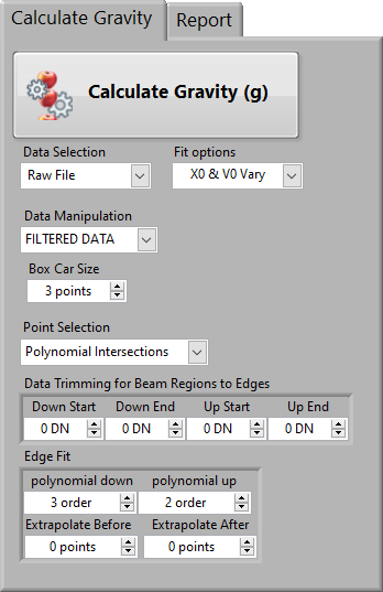
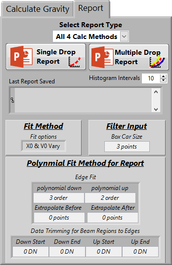
The lower left region contains a tab control with two visible tabs named “Calculate Gravity” and “Report” as well as one hidden tab named “*single States”. This is hidden for ease of use and can be accessed by right clicking on the tab and selecting “Unlock Super User Tab” doing this will result in a fun Easter Egg. The audio can be silenced when un-hiding this tab by holding down shift while selecting the right click option.

On the “Calculate Gravity” tab there is a single push button named “Calculate Gravity (g)” which utilizes 4 pull down controls named Data selection, Fit options, Data Manipulation, and Point selection. These pull-down controls define the steps taken to analyze the data and calculate gravity. The function of each of these pull-down controls is described below.
The Data selection pull-down control is defaulted to “Raw File” which means the data used to calculate gravity will come from the selected file in the multi-column list-box.
When the Data selection control is set to “Clipboard points”, the clipboard is expected to contain time(sec) and distance(mm) measurements from a user created drop experiment.
When the “Calculate Gravity (g)” button is pushed, the points in the clipboard will be fitted to a parabola to utilizing the Fit options pull down menu options. The resulting gravity calculation will be shown in the “FIND GRAVITY” tab
The expected clipboard format is as follows:
- It must contain a set of at least 3 human readable points.
- The points must be formatted as two columns of time(sec) and distance (mm) that are tab delimited with an end of line character after each point.
- If any letters from A to Z are found in a row that row is ignored.
The Data Manipulation and Point selection options only operate on raw drop data from the Gravity Lab. Therefore, they are automatically hidden when the Data Selection control is set to “Clipboard points”.

The Fit options pull-down control determines the coefficient constraints for fitting the selected data points to a parabolic curve using a Least Square Singular Value Decomposition(SVD).
The data points that are fitted to a parabolic curve are determined by selected by the other 3 pull down controls.
By default the starting position(X0) and the starting velocity(V0) are allowed to vary “X0 & V0 Vary“. For the gravity lab, the tightest data spread that is also nearest the expected gravity results from choosing the a starting velocity(V0) equal to zero, i.e. the “V0 = 0” option.
The Data Manipulation Pull-down control determines if the data is filtered or raw before the laser beam crossing points to be fit are found.
The default option is “RAW DATA”, and when it is changed to “FILTERED DATA” a control named “Box Car Size” becomes visible.
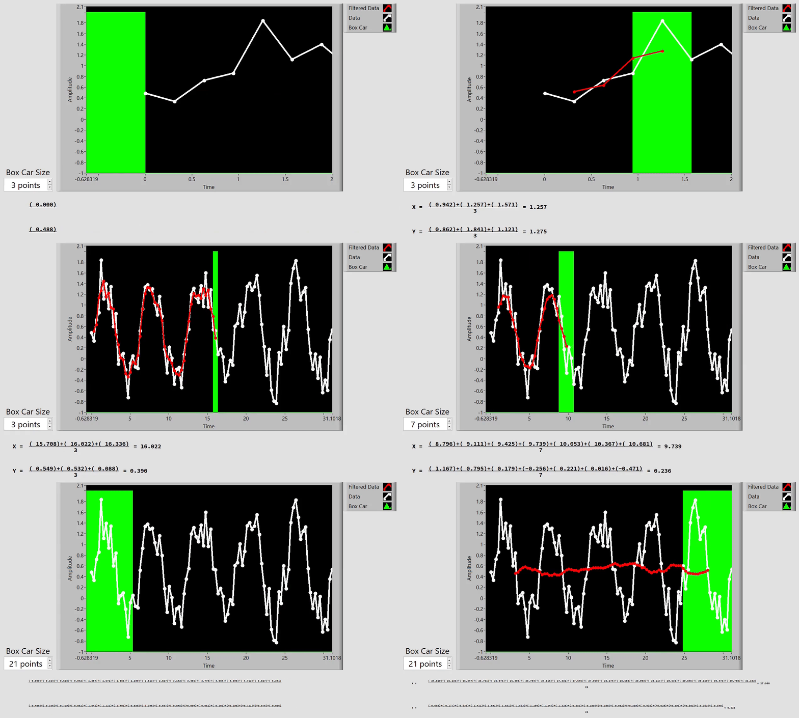
This control determines the size of the “box car” window to be used for smoothing the data. A box car filter works by averaging each point in the raw with its nearest neighbors as determined by the box car size. This has the effect of reducing large spikes in the data than can throw off a minimum value search.
The values you can insert into this are limited to even numbers to keep the data from shifting in time when the averaging occurs. The total data set reduces in size by a value of the box car size – 1. This is split evenly on the front and end of the data set.
The Point selection pull-down control determines how the Laser Beam crossing points are found.
The “Simple Minima” method searches for a minimum associated with each expected beam position.
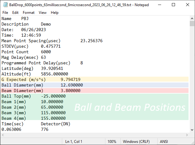
The expected minima locations come from the “Ball Top(mm)” and “Beam #(mm)” values listed in each data file header.
The “G Expected (m/s^2)“ value is used to calculate a search window around each beam position in units of seconds.
The search window is sized by the “Ball Diameter“ before the expected minima and the laser “Beam Diameter” after the expected minima.
The “Polynomial Intersections” method determines the minima at each expected beam position by fitting a polynomial equation to data on either side of the found minima.
The data that is being fit on either side of the found minim is set by the search window mentioned above, the “Data Trimming for Beam Regions to Edges” control and the “Edge Fit” control.
When the polynomial equations are found for each side of the minima, they are set equal to each other and their “roots” are determined. The “root” value nearest the minima is chosen as the beam crossing point.
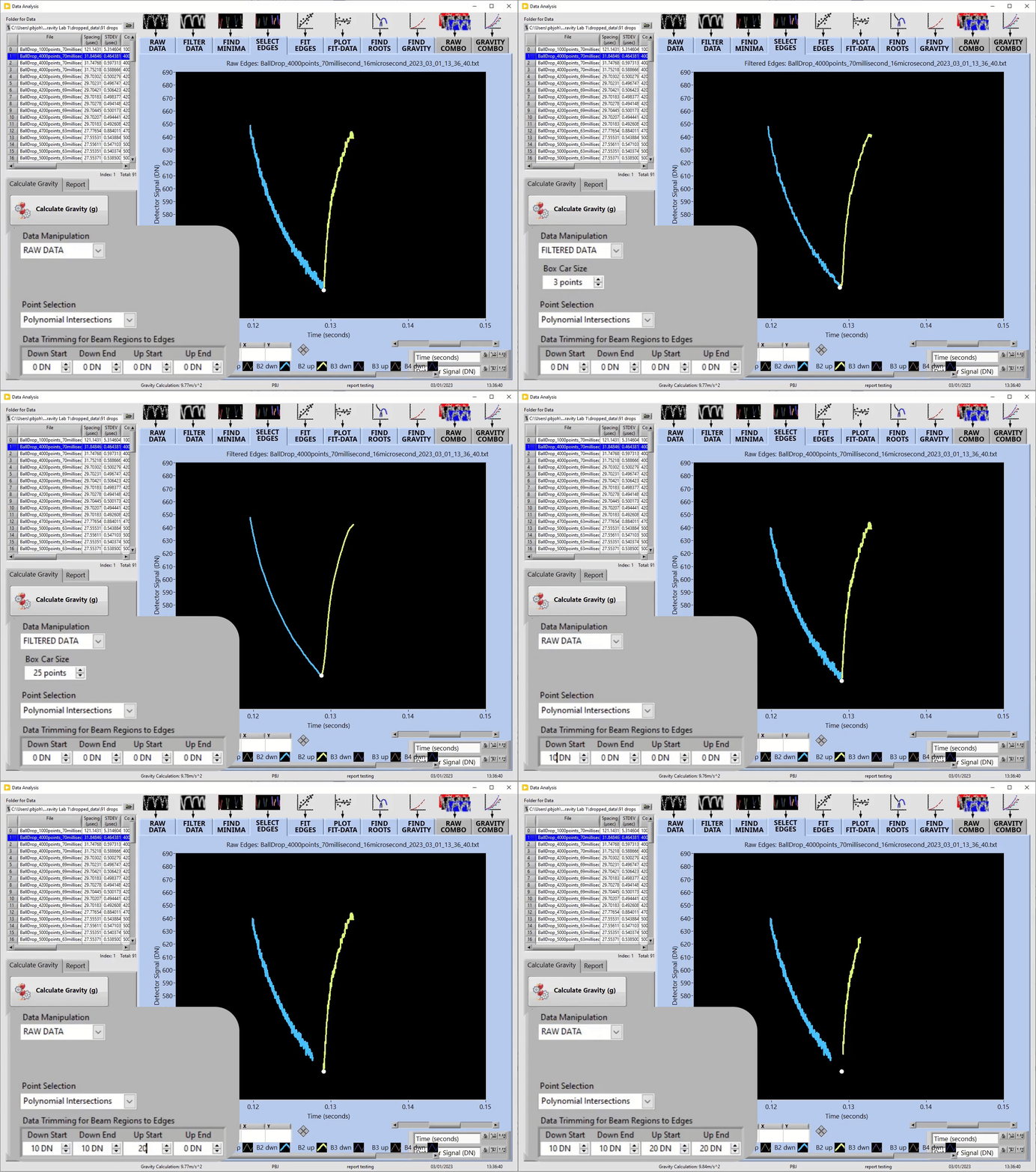
The “Data Trimming for Beam Regions to Edges” control allows you to trim the points used for fitting the polynomial on each side of the found minima.
The “Down Start” and “Down End” inputs trim the beginning and end of the first edge which is moving down toward each minima.
The “Up Start” and “Up End” inputs trim the beginning and end of the second edge which is moving up after the minima.
The Trimming of each edge is determined by the offset in value given in DN from the Minima or Maxima in each edge. The data is kept continuous by finding the first value to meet these criteria when moving in a forward or backwards direction on each line.
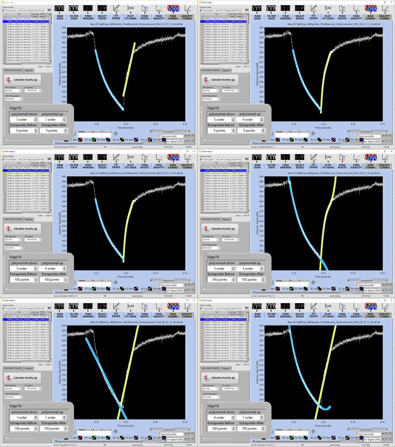
The “Edge Fit” control allows you to select the polynomial order used to fit each side of the line. I have found that a 3rd order for “polynomial down” and 4th for “polynomial up” provides the best data fit. The “Extrapolate Before” and “Extrapolate After” options are purely for visualizing the polynomial fit as seen in the Fit Edges Tab.
On the “Report” tab there are two push buttons named “Single Drop Report” and “Multiple Drop Report”. These buttons create unique PowerPoint reports that summarize the gravity calculation(s). They both use the “Select Report Type” pull-down control to and the relevant input values from the “Calculate Gravity Tab” to determine what data goes into the report. These input values are displayed as indicators on this tab, but are controlled on the “Calculate Gravity” Tab. The “Last Report Saved” indicator displays the file and path of the last report saved. You can quickly open the folder or PowerPoint using its right click options named “explore folder” and “open file” respectively.

The “Single Drop Report” button creates a PowerPoint of the currently selected drop data file in the multi-column list-box.
Each of the 4 individual selections of the “Select Report Type” control will create a PowerPoint report with the following format.
- The summary of the gravity calculation results.
- The calculation inputs.
- The summary of the raw data used.
When “All 4 Calc Methods” is selected the PowerPoint will consist of 13 slides that combine the summaries and calculated inputs for the 4 methods of “Raw Minima”, “Filtered Minima”, “Raw Poly Fit”, and “Filtered Poly Fit”. Just like the individual summaries, the last is a summary of the raw data used.

The “Multiple Drop Report” button creates a PowerPoint of all the dropped data files in the in the multi-column list-box. The “Histogram Intervals” control determines the number of bins used in the Histogram plots.
Each of the 4 individual selections of the “Select Report Type” control will create a PowerPoint report with the following format.
- The summary of the gravity calculation results with inputs used
- Histogram for Gravity, Distance and Time calculations
- A zoomed in image for given beam crossings.
- Equations for each gravity calculation.
- A plot of all the raw data used.
- A list of all the file names for the raw data.
When “All 4 Calc Methods” is selected the PowerPoint will contain slides for sections 1) through 4) for each of the 4 methods of “Raw Minima”, “Filtered Minima”, “Raw Poly Fit”, and “Filtered Poly Fit”.


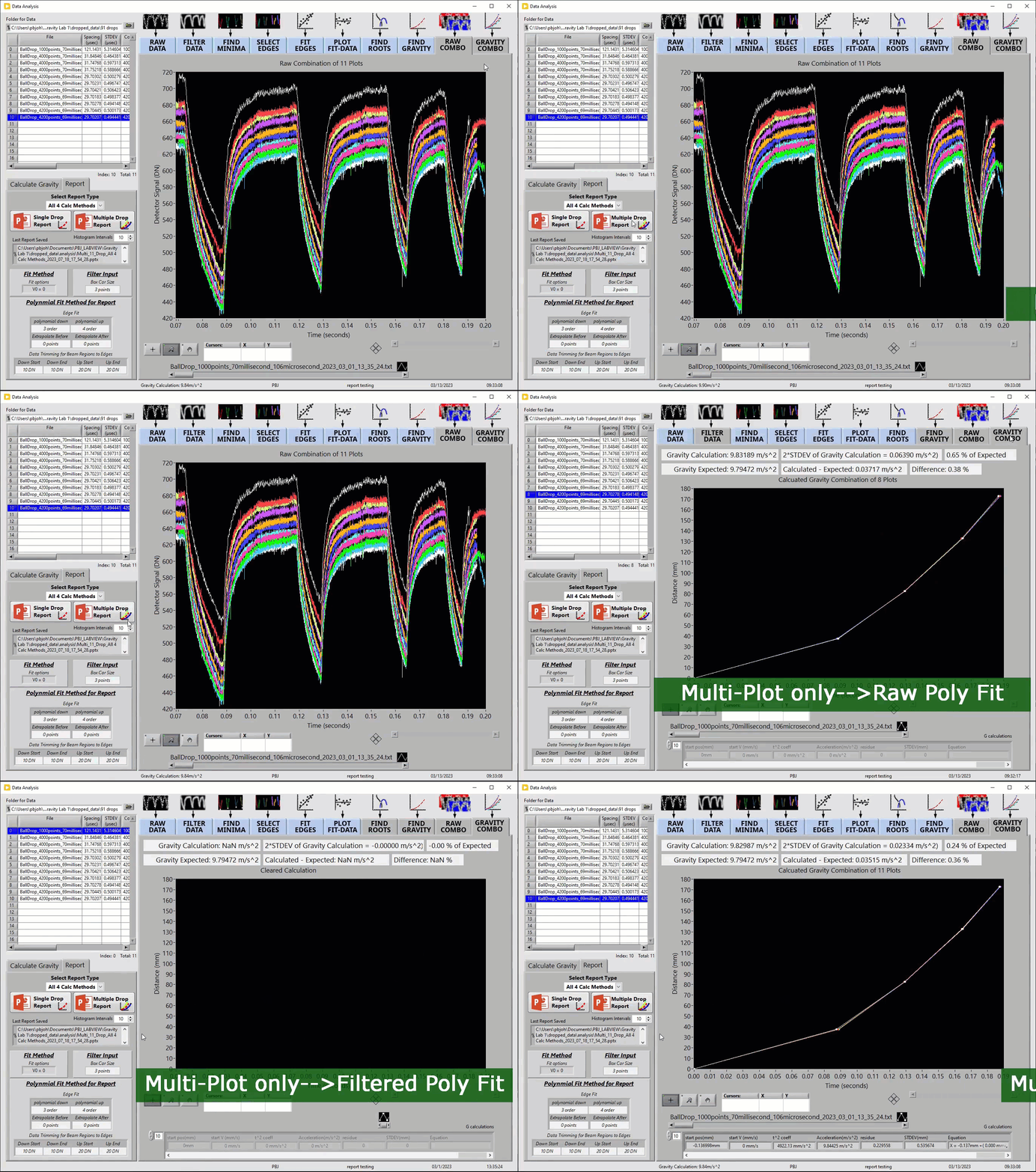
To avoid creating a PowerPoint, you can right click on the “Multiple Drop Report” button and select one of the 4 options “Multi-Plot only –> Raw Minima”, “Multi-Plot only –> Filtered Minima”, “Multi-Plot only –> Raw Poly Fit”, and “Multi-Plot only –> Filtered Poly Fit”
This is useful for quickly understanding the variability of the gravity calculation results summarized in the “GRAVITY COMBO” tab.
Graphing Region
Two thirds of the “Data Analysis” window displays 10 unique plots located in a tab control.
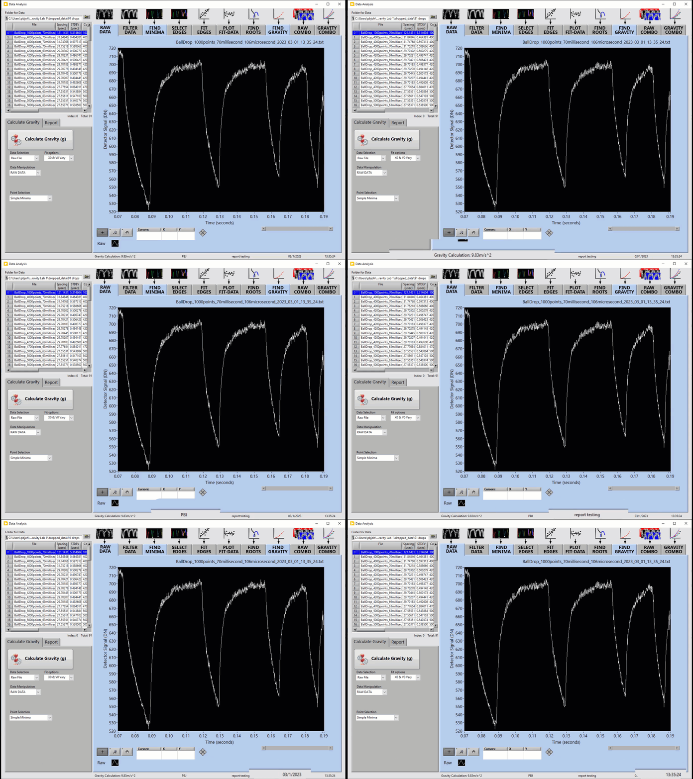
Directly below the tab control information is displayed for each file selected in the multi-column list-box.
When the Calculate Gravity (g) button is pushed, the resulting calculation is shown in two places, below the tab control and inside the “FIND GRAVITY” tab.
To the right of the gravity calculation below the tab control is the tester name, the test description, the date of the test and the time the test was taken. These are all pulled from the header in the highlighted data file in the multi-column list-box.
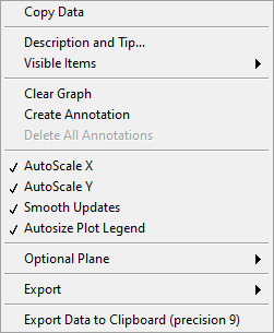
Every plot in the Data Analysis window has an extra right-click option named “Export Data to Clipboard (precision 9)”. This option allows you to export all the data in the current plot such that you will always have 9 digits past the decimal point. This is useful, because the default LabView export to clipboard utilizes the displayed precision on the plot. See my post on “LabView – XY Graphs” for details on how to access any data point and create tailored image captures. This post is useful for any program written in LabView that uses XY Graphs.
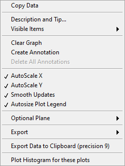
The plot found on the “GRAVITY COMBO” tab has an additional right-click option named “Plot Histogram for these plots”.
This option opens the “Histogram Plots” window which allows you to plot Histograms for all the gravity calculations in this plot, as well as a histogram for each beam crossing point in units of time or distance.
The “Plot Selection” and “Unique Position Type” pull down controls determine what histogram is being displayed.
To display the gravity calculations histograms set the “Plot Selection” pull down control to “Gravity Calcs”
To display the time measurement histograms set the “Plot Selection” pull down control to one of the unique distances and select “Time Found (sec)” from the “Unique Position Type” pull down control.
To display the distance fit histograms set the “Plot Selection” pull down control to one of the unique distances and selection “Position Fit (mm)” from the “Unique Position Type” pull down control.
